Some perspectives on the Yoneda lemma
With the power of geometry, anything is intuitable.
Every once in a while I find myself thinking about the Yoneda lemma in a slightly new way from what I knew before. In this post I collect some beautiful conceptual perspectives on Yoneda that I find particularly enlightening:
- “Probing” spaces, in algebraic topology and homotopy theory.
- “Generalized spaces”, in algebraic geometry and sheaf theory.
- “Function extensionality” and “generalized elementary reasoning”, in categorical logic.
- (One bonus perspective, using Kan extensions & coends).
I wanted the post to be appealing also to people without too much background in category theory, so the first section spends some time introducing some motivating examples for functors and natural transformations.
Be warned that I got a little carried away in some parts, so feel free to skim / skip ahead!
The perspective of probing
One of the basic constructions in algebraic topology is the fundamental group of a space, denoted by $\pi_1(X)$. Roughly speaking, this is the collection of all “loops” in the space $X$. You can think of a loop as a point, wandering around the space for a while, until finally going back to where it started. I like to think of these as “animations”, happening dynamically over time.
$\pi_1(X)$ is a group under concatenation of loops, i.e. “composition of animations” (play one animation after the other). There’s some subtleties related to homotopies between loops, but that’s irrelevant for our current discussion.
We say $\pi_1$ is a functor, because it not only maps spaces to their groups of loops, but also given a function between spaces it can tell you how loops transform. Indeed, you can just take each “frame” of your “animation” and pass it through the function.
But in fact $\pi_1$ is a very special functor, because it is representable. This means it has the form $\pi_1(X) \iso \Hom(S,X)$ where $S$ is some object and $\Hom$ is the collection of functions from $S$ to $X$ (again, ignoring homotopy-related subtleties). Such isomorphism also has to be natural, in the sense that it also matches how both sides act on functions between spaces, not just spaces themselves.
The fundamental group is thus a way to probe complicated spaces with a more well-understood one. Many invariants in algebraic topology arise this way.
It’s not too hard to guess what this representing object may be – it’s the circle $S = S^1$. In some sense, the circle is a “generic” loop, and every other loop in any other space is modeled on this one. More precisely, $S^1$ contains a “universal animation” of a point going around the circle once (say, counter-clockwise). Then if $\gamma \in \pi_1(X)$ is a loop in $X$, then you can always find some continuous function $f:S^1 \to X$ through which the universal animation will become $\gamma$.
Remark: You may be thinking I overcomplicated my explanation here – rather than picturing loops inside $S^1$, why not just think of $S^1$ itself as the loop? This is intentional. The “universal loop” that I describe is precisely the loop given by the identity function in $\Hom(S^1,S^1) \iso \pi_1(S^1)$ – that’s gonna pop up repeatedly later on.
So far I’ve just introduced the functor $\pi_1$, and the fact that it’s representable. To state the Yoneda lemma we are missing one more piece: natural transformations. A natural transformation between two functors $F,G$ is essentially a function $\alpha : F(X) \to G(X)$ for every $X$, whose definition doesn’t actually depend on the “internal structure” of $X$. The most classical example is from linear algebra:
Example: There is a linear map $\alpha : V \to V^{**}$ from any vector space to its double-dual. I claim that this is a natural transformation (from the identity functor to the double-dual functor). This $\alpha$ is defined as follows:
\[\alpha(v) := (\psi \mapsto \psi(v))\]In words, $\alpha$ sends every vector $v$ to the “evaluation at $v$” functional, which is itself defined on functionals.
As you may have heard, if $V$ is finite dimensional, this $\alpha$ becomes an isomorphism.
Well, big whoop, right? Clearly $V$ and $V^*$, and even $V^{**}$, they all have the same dimension. So they are automatically gonna be isomorphic: choose a basis for each one, and define isomorphisms by sending one basis to another.
The problem is that such isomorphism is not natural – it depends on the internal structure of the vector space, namely, your particular choice of basis vectors. In contrast, $\alpha$ defined above does not rely on any basis. It’s defined by the same formula, regardless of the vector space $V$, its dimension, the field that it’s defined over, etc. This is what makes $\alpha$ “natural”. Of course category theory provides a rigorous sense for naturality, which you can find in any textbook (I must recommend Riehl’s).
Now that we know about natural transformations, let’s get back to topology. Here is a toy example in topology for an operation one might consider on fundamental groups: $\alpha : \pi_1(X) \to \pi_1(X)$, defined on any loop by running its “animation” twice in a row. A sort of loop doubling operation, if you will.
This operation is completely “natural” in the sense that it doesn’t depend on any special features of $X$. In fact the exact same definition works for any space $X$ whatsoever. But hey, if the functor $\pi_1$ is represented by a “universal loop”, shouldn’t this doubling operation also be represented by some “universal doubling”? And indeed it is! There is a function $f : S^1 \to S^1$ which wraps the circle once around itself. Now given any loop in any space $\gamma \in \pi_1(X)$, identify it with a map $\gamma \in \Hom(S^1,X)$ as above, and compose this $\gamma$ with $f$:
\[S^1 \xrightarrow{f} S^1 \xrightarrow{\gamma} X\]This gives a new loop. Clearly, every other map from $S^1$ to itself will give a similar operation on loops in arbitrary spaces.
More generally, given any representable functor $F \iso \Hom(c,-)$ and any morphism $f:d\to c$ in your category, you very naturally obtain a natural transformation $f^* : \Hom(c,-) \to \Hom(d,-)$ by composing with $f$. This composition is natural because it’s completely independent of any particular properties of the map $\gamma$ that you’re applying it on.
Now we can finally state our first version of the Yoneda lemma, which is a minor weakening of the general case that we shall see later.
Yoneda lemma (weakened form): The assignment of morphisms $f$ to natural transformations $f^*$ is a bijection:
\[\Hom(d,c) \iso \rm{Nat}(\Hom(c,-),\Hom(d,-))\]Above we’ve seen how to go from the LHS to the RHS. Conversely, given any natural transformation of the form
\[\Hom(c,-) \to \Hom(d,-)\]Specialize this to the specific object $c$. You get a function
\[\Hom(c,c) \to \Hom(d,c)\]Lastly just take the image of the identity morphism $\id_c$, and voila, you get the same $f:d\to c$ you started from (exercise: verify this). Even if you didn’t start from $f$ but directly with some natural transformation, the Yoneda lemma says that there must be some morphism $f$ between the representing objects which induces your given natural transformation.
Note there is also a “coYoneda lemma” for contravariant functors, those of the form $\Hom(-,c)$.
This interpretation is very nice, and it can actually be pushed even further. I will briefly discuss some deeper ideas in algebraic topology that I find very intriguing; though if you feel satisfied with everything above feel free to skip ahead to the next section.
So, we’ve seen how the loop doubling on $S^1$ induces a similar operation on all loops in all spaces. Certainly, you could also define loop tripling, quadrupling, and so on. Or you can define a “negation” function which plays your animation in reverse – this corresponds under Yoneda to the animation of going once around $S^1$, but this time clockwise. It smells like there’s some algebraic structure to be found here.
Most generally, let us consider the space $S^1\vee S^1$ obtained by welding two circles together at a single point. There is an “animation” $\mu : S^1 \to S^1\vee S^1$ of a point: start at the contact point, go once around the first circle, then go once around the second circle. This may be thought of as the universal composition of animations. Indeed, the functors & natural transformation represented by $\mu$ is
\[\mu^* : \Hom(S^1\vee S^1,-) \to \Hom(S^1,-)\]If you identify a function from $S^1\vee S^1$ with a pair of functions from two copies of $S^1$, you can rewrite this as
\[\mu^* : \Hom(S^1,-)\x\Hom(S^1,-) \to \Hom(S^1,-)\]And that’s precisely the multiplication that makes each $\pi_1(X)$ into a group! So in fact, not only each $\pi_1(X)$ is a group, but actually $\pi_1$ itself is a group object in the category of functors & natural transformations! By the Yoneda philosophy, any kind of structure on a representable functor should be “pulled down” to a universal structure on the representing object.
Indeed, $S^1$ forms what’s called a cogroup object in the homotopy category: it admits a comultiplication map $\mu : S^1\vee S^1\to S^1$, a coinversion map $\iota : S^1 \to S^1$, and a counit map $\eps : S^1 \to pt$. These “co” maps satisfy all the axioms of a group, but in reverse: $\mu$ is “coassociative”, $\eps$ is “counital”, etc. It’s even true that the “loop doubling” map is a cogroup homomorphism, which automatically makes the induced operation on fundamental groups a group homomorphism. I’ll leave the details for you.
Edit: As was pointed out to me by a reader who, unlike myself, actually did think through the details more carefully, this is certainly NOT a (co)group homomorphism! In general the ``power’’ function $g \mapsto g^n$ is only a homomorphism if $n=0,1$ or if the (co)group is abelian. But it’s still a function between the underlying sets, and I think it gives a nice geometric picture to have in mind.
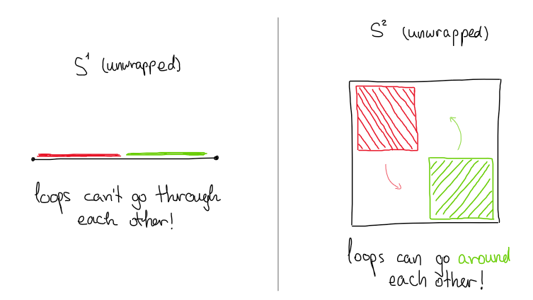
Similarly any sphere $S^n$ forms a cogroup object, and the functors they represent are precisely the higher homotopy groups $\pi_n$ which are also groups, consisting of higher dimensional loops & compositions between them. You can think of those higher dimensional loops as animations with “multiple time parameters”, though this intuition is starting to get sketchy. A special thing that happens in the higher homotopy groups is that they become abelian. Why? Let’s apply our Yoneda philosophy: we need to show that the cogroup $S^n$ for $n\geq 2$ is “cocommutative”. Without diving into precise definitions, this can be seen through the following drawing:
The curious reader may look up the Eckmann-Hilton trick for more on that, and the little cubes $\mathbb{E}_\infty$-operad for a vast generalization of commutativity in terms of higher dimensional configuration spaces.
You can actually exploit the Yoneda philosophy to represent even more complicated structures. Consider the following diagram
Here $\Delta^n$ is the standard topological $n$-simplex; so $\Delta^0$ is a point; $\Delta^1$ is an interval; $\Delta^2$ is a triangle; $\Delta^3$ a tetrahedron, etc. The maps shown are “face maps”: the interval has two endpoints, the triangle has three sides, the tetrahedron has four faces. One can also define maps going in the opposite direction, known as “degeneracy maps”, and the resulting configuration of objects & morphisms is known as a cosimplicial object – cosimplicial topological space, in our instance. Now here’s a tease for your curiosity: this specific cosimplicial object may reasonably be called an “$\infty$-cogroupoid object” in the category of topological spaces. The functor it represents sends every topological space to its underlying $\infty$-groupoid, also known as its simplicial nerve, also known as its singular complex. Various natural operations between those $\infty$-groupoids are, as predicted by the Yoneda lemma, going to be represented as operations on the universal $\infty$-groupoid we’ve just seen.
All this is fairly abstract, and frankly not at all useful in practice, besides being fun to think about. You really know you’ve gone too abstract when you start a paragraph with “the triangle has three sides” and end it with $\infty$-groupoids.
The perspective of generalized spaces & moduli problems
Abstract nonsense aside, it’s time to look at the next interpretation of the Yoneda lemma. Suppose $\mathbf{Aff}$ is some category of “affine objects”:
- If you care about algebraic geometry, these may be affine varieties / affine schemes.
- If you care about differential geometry, these may be open subsets of $\mathbb{R}^n$.
- If you care about complex geometry, they could be open domains in $\mathbb{C}^n$.
A “space” $X$ in each of these contexts is supposed to somehow be obtainable from gluing affine patches together. We can encode this gluing data in a presheaf, i.e. a functor from $\mathbf{Aff}^{op}$ to the category $\mathbf{Set}$ of sets:
- For each affine patch $A$, the set $X(A)$ should tell you all the pieces of type $A$ that were used in constructing $X$.
- For each inclusion $A \into A’$ of affine patches, the function $X(A’) \to X(A)$ should tell you which smaller pieces are glued to which larger pieces.
Of course every affine space $A\in\mathbf{Aff}$ gives such functor, namely $\Hom(-,A)$. I will also denote this functor by $\yo_A$, with the squiggly Hiragana letter $\yo$ (“yo”). Typically not all spaces are affine. That is, not every presheaf is representable. But that’s actually a good thing, it means that we can form a “category of generalized spaces” $\PSh(\mathbf{Aff})$ and an “embedding” $\yo : \mathbf{Aff} \to \PSh(\mathbf{Aff})$.
Now suppose $X$ is a presheaf – a generalized space. We wanna be able to see all the affine patches contained inside it. But now there are two reasonable ways to do so:
- By definition, the patches of type $A$ appearing in $X$ are just those obtained by evaluating the functor $X$ on the object $A$. This is $X(A)$.
- More geometrically, we’d like to just look at literal maps from the (affine) space $A$ to the (genralized) space $X$. Using the embedding above we can actually bring these two to the same category, and hence take the homset between them: $\Hom(\yo_A,X)$.
So which is the right answer? $X(A)$? Or $\Hom(\yo_A,X)$? it turns out that the stars are aligned, and everything works out: these answers are the same.
Yoneda lemma (full version): $\Hom(\yo_A,X) \iso X(A)$.
One of the main consequences of this (whose proof is left as an easy exercise) is:
Corollary: The Yoneda embedding $\yo : \mathbf{C} \to \PSh(\mathbf{C})$ is a faithful functor (the functorial analogue of injectivity).
Note also that every affine patch $A$ is definitely expected to appear inside itself. This is gonna be the element in $\yo_A(A)$ corresponding to the identity transformation in $\Hom(\yo_A,\yo_A)$. More generally:
Corollary: If $A,A’$ are affine spaces then, applying the Yoneda lemma with $X=A’$, we obtain
\[\rm{Nat}(\Hom(-,A),\Hom(-,A')) \iso \Hom(A,A')\]which looks a lot more like the weakened version we’ve seen earlier.
Usually generalized spaces are a bit too general, so much so that they kind of lose some interesting geometric aspects. In practice we would often restrict our attention to a more well-behaved subcategory of functors, for instance, those functors that actually arise from honest to god manifolds.
In the context of algebraic geometry, unlike differential geometry, the functorial perspective on schemes is much more prominent. Indeed a scheme is nothing but a presheaf which satisfies some form of “descent condition” (Zariski descent, to be precise), also known as a sheaf.
Nowadays it’s very common to work in even larger subcategories, especially when working with moduli problems. A “moduli problem” is nothing but a presheaf $\mathcal{M}$ which sends each space to some set of geometric objects associated to this space: this could be the set of vector bundles, principal bundles, families of curves, etc. Then much of moduli theory becomes a game of compromise: on the one hand you want to find a large enough subcategory which contains all the interesting moduli problems, but you also don’t wanna make it too large and lose important geometric properties. You can also think about this in terms of representability: not any presheaf on schemes is representable by a scheme, but it might be representable by an object in your larger subcategory.
Another important direction of generalization is, instead of $\mathcal{M}$ sending each space to a “set” of geometric objects, send it to a “set with equivalence relation” of geometric objects, aka a groupoid. For instance, you may send each space to the groupoid of vector bundles and isomorphisms between them. Again the full category might be too large for geometric purposes, so you’d often want to restrict yourself to some well-behaved subcategory such as algebraic stacks, Artin stacks, etc. And, just as working on a manifold can be done locally on affine patches, so can working on a stack be done locally on affine schemes mapped into it.
This approach is much more successful than working with mere sets, and turns out that even more moduli problems become representable upon this extension. Going even further, you can take your moduli problem $\mathcal{M}$ to be valued in $\infty$-groupoids, and get even richer results. And it’s all thanks to the Yoneda lemma.
The perspective of function extensionality
When working in a category, you don’t always have access to “elements” like in the category of sets, abelian groups, etc. So in general, you need to be more careful, and make your proofs using diagram chasing. I like to call such proofs “non-elementary”, not because they are necessarily more complicated, but just because they circumvent the use of elements.
Nevertheless, there are still ways to simulate elements, even in arbitrary categories, and writing “elementary-like proofs” using those.
Definition: Let $\mathbf{C}$ be a category and $C \in \mathbf{C}$ an object. Let $X \in \mathbf{C}$ be another object. Then a generalized element / generalized point of shape $X$ is a morphism $X \to C$.
This definition is closely related to the functorial description of schemes from the previous section. In fact the underlying functor of a scheme is actually called its “functor of points”, and rather than speaking of “affine patches” you would usually just speak of points built from various rings.
As an instructive example, if $\mathbf{C}$ is the category of sets, then you can take $X$ to be the singleton set $\mathbb{1}$, and then $\mathbb{1}$-shaped elements of a set are exactly the usual elements. In this example, every set $X$ can be written as a disjoint union of many copies of $\mathbb{1}$, so the generalized elements of shape $X$ don’t really add any new information beyond what $\mathbb{1}$ can see. Of course not every category has this feature.
Let’s see some applications of generalized elements. Recall that a function $f:C\to D$ between sets is called injective if it only sends equal inputs to equal outputs (i.e. unequal inputs necessarily give unequal outputs):
\[f(x)=f(y) \Thus x=y\]where $x,y\in C$.
Now suppose $f:C\to D$ is a morphism in some category. An $X$-shaped generalized element of $C$ is nothing but a morphism $x : X \to C$, and to “evaluate” a morphism on a generalized object we simply compose: $f\circ x$. Note that the result of evaluation is also a generalized object, of the same shape as the original. To ease our eyes, we can even denote composition by juxtaposition, without the little circle, and simply write $fx$. I hope you can see where I’m going with this…
The analoguous notion of injective functions in category theory is monomorphisms. These are defined by a universal property: $f$ is monomorphic if, for all objects $X$ and all morphisms $x,y : X \to C$, if these morphisms satisfy $f\circ x = f\circ y$ then $x=y$. Written differently,
\[fx = fy \Thus x=y\]That’s injectivity! Now the universal property doesn’t seem so scary anymore.
Finally, let’s see a more advanced example. One of the ZFC axioms in set theory is the axiom of extensionality, which says that two sets are equal if and only if they contain the same elements. Consequently, we get the property of function extensionality (which may also be taken as an axiom, in more exotic foundational systems). This says two functions are equal if and only if they return equal outputs for equal inputs:
\[\forall x, f(x) = g(x) \Thus f=g\]We’d like to use a similar strategy to prove equality between morphisms in a category. Fix two objects $C,D$ and two morphisms $f,g:C\toto D$ between them.
Theorem: If $fx=gx$ for all $x:X\to C$ then $f=g$.
Proof: Using the Yoneda embedding, we have two presheaves $\yo_C = \Hom(-,C)$ and $\yo_D = \Hom(-,D)$, along with two natural transformations between them $\yo_f,\yo_g : \yo_C \toto \yo_D$. If you think through the definitions, you may notice that $\yo_f$ is precisely the evaluation on generalized elements: it takes $x:X\to C$ and returns $fx:X\to D$. Likewise for $\yo_g$. Moreover this evaluation process is natural in the sense that it does not depend on any specifics of the shape $X$.
Recall that by the Yoneda lemma, $\yo$ is faithful, so proving $f=g$ is the same as proving $\yo_f = \yo_g$, and this is the same as proving $\yo_f(X) = \yo_g(X)$ for all shapes $X$. But that’s exactly our assumption! $\square$
Remark: In the last step of the proof we implicitly relied on function extensionality for each component of the two natural transformations, i.e. the actual set-level functions $\yo_f(X),\yo_g(X) : \yo_C(X) \toto \yo_D(X)$. So really the only reason function extensionality works is because it holds in $\Set$. Likewise, most reasonable properties of $\Set$ would be inherited by presheaf categories. Such categories of presheaves (and their subcategories) are called topoi (plural of topos).
I wrote another blogpost where I use both elementary techniques and diagram-chasing (and some fancier techniques) to prove a standard result in homological algebra:
Bonus perspective - co/ends & the density theorem
Here is a crash course on Kan extensions and co/ends.
Suppose $F:\mathbf{D} \to \Set$ is a certain diagram of sets. Recall that the limit of $F$ is a certain subobject of the product $\prod_D{F(D)}$ over all objects in the diagram, while the colimit is a certain quotient of the disjoint union $\coprod_D{F(D)}$.
Kan extensions are supposed to generalize this in the following sense: suppose you have a functor between diagrams $p:\mathbf{D} \to \mathbf{E}$ and a diagram of sets $F:\mathbf{D}\to\Set$. The goal is to define a new diagram $F’:\mathbf{E}\to\Set$ whose value on the object $E$ is the “relative” co/limit of the subdiagram of $\mathbf{D}$ consisting only of those objects that are “above” $E$, in a sense which I won’t make precise (it’s not quite the naïve fiber $p^{-1}(E)$). This of course must include various compatibility requirements between those different results, and it must somehow be made functorial.
You can think about this process as “integration along fibers”, except that integration now comes in two flavors; either limit-ish integration or colimit-ish integration. You can think of the colimit-ish integration as integration “with compact supports” and the limit-ish one as general integration. As an example, keep in mind infinite co/products of abelian groups: $\coprod_i{A_i}$ is only allowed finitely many nonzero components, while $\prod_i{A_i}$ is allowed infinitely many nonzero components. if $i$ ranges over a finite set then the two become equivalent, and commonly denoted as a direct sum $\bigoplus_i{A_i}$.
Correspondingly, there are two types of Kan extensions: the right Kan extension $\Ran_pF$ which is more limit-ish and the left Kan extension $\Lan_pF$ more colimit-ish. The actual definition can be found in any text on category theory, but for my purposes just the intuition will suffice.
To demonstrate how Kan extensions are “integration along fibers”, let’s consider the case where there is only one fiber, i.e. $\mathbf{E} = \mathbf{1}$ is the one-object category, and $p:\mathbf{D}\to\mathbb{1}$ is the unique functor to it. Then, working through definitions, $\Ran_pF$ indeed coincides with $\lim F$ and $\Lan_pF$ coincides with $\colim F$. If you’re a fan of algebraic geometry, there is even more suggestive notation for these: $\Ran_pF$ is often denoted by $p_*F$ and $\Lan_pF$ is denoted by $p_!F$. This is supposed to convey the intuition that you’re “pushing forward” your diagram along $p$, once with compact supports and once with general support. And as you might expect, there is also a restriction functor $p^*$ fitting into the usual adjunctions
\[p_! \dashv p^* \dashv p_*\]Here are my two favorite example of Kan extensions (strictly speaking, the first one is not a Kan extension between ordinary categories but only between $\infty$-categories, or even just $2$-categories):
Example 1: There is a functor $\Modu : \CRing \to \Cat$ which sends each commutative ring to its category of modules. There is also a functor $\Spec : \CRing^{op} \to \Sch$ which sends every commutative ring to the associated affine scheme. In algebraic geometry, rings are to modules as schemes are to quasicoherent sheaves. Namely a qcoh sheaf on a scheme is a sheaf which, locally on each affine patch, looks like a module. In other words a qcoh sheaf sort of looks like a “limit-ish integral” of modules over all the affine patches in a scheme. Based on this you might expect some right Kan extension to fit into this mix, and yes it does! The functor $\QCoh : \Sch \to \Cat^{op}$ which sends a scheme to its category of qcoh sheaves is precisely the right Kan extension $\Ran_{\Spec}\Modu$ of the module-category-functor along the $\Spec$ embedding.
This example should remind you the perspective of generalized spaces discussed earlier. In fact if you identify schemes as generalized spaces over $\Aff\Sch \equiv \CRing^{op}$, then the functor $\Spec$ agrees with the Yoneda embedding, which sends each affine scheme to the corresponding generalized space.
Before giving the second example, I must briefly talk about simplicial sets. We’ve already encountered simplicial spaces in the first section of this post, and simplicial sets are very similar. In fact we can even use the second perspective, of generalized spaces, to get some better intuition for those.
This time the “affine patches” that our spaces are built out of will be simplices (points, lines, triangles, and their higher dimensional versions). These live in a simplex category $\mathbf{\Delta}$ which has one object $\Delta[n]$ for each natural number $n$, and all the face & degeneracy maps between them. The standard cosimplicial object in topological spcaes, which we’ve seen earlier, is a covariant functor $\rm{st} : \mathbf{\Delta} \to \Top$.
Now a simplicial set should be something built out of those simplices. So by the philosophy of generalized spaces, a simplicial set should be an object of the presheaf category $\sSet := \PSh(\mathbf{\Delta})$, i.e. a contravariant functor $F : \mathbf{\Delta}^{op} \to \Set$. The value of this functor on $\Delta[n]$ is the set of all $n$-simplices in your generalized space.
Example 2: Every abstract simplicial set should be realizable concretely as a topological space, simply by taking one standard simplex $\Delta^n$ for each element of the set $F(\Delta[n])$, and gluing them together appropriately. This “gluing together” might make you think there’s some “colimit-ish integral”, i.e. some left Kan extension, involved, and yes there is! The geometric realization functor $|-| : \sSet \to \Top$ is the left Kan extension of the standard cosimplicial space $\rm{st} : \mathbf{\Delta} \to \Top$ along the Yoneda embedding $\yo : \mathbf{\Delta} \to \sSet$.
I also promised co/ends, and although their general definition is outside the scope of this post, they do specialize to Kan extensions and make the notation much nicer. So if you’re unfamiliar with them, you can take the following isomorphisms as the definitions of the RHSs (ends and coends, respectively):
\[\Ran_pF \iso \int_{D\in\mathbf{D}}{\Hom(\mathbf{E}(-,p(D)), F(D))}\] \[\Lan_pF \iso \int^{D\in\mathbf{D}}{\mathbf{E}(p(D),-)\x F(D)}\]The first formula can be written a bit nicer using the Yoneda embedding
\[\Ran_pF \iso \int_{D\in\mathbf{D}}{\Hom(\yo_{p(D)},F(D))}\]and the second can be rewritten using the “contravariant” Yoneda embedding (defined by $\Hom(A,-)$, instead of $\Hom(-,A)$):
\[\Lan_pF \iso \int^{D\in\mathbf{D}}{\yo^{p(D)}\x F(D)}\]These notations really drive home the intuition as integration: for a right Kan extension, you take the “limit-ish” integral over all the affine patches that map into $F$ (like in the first example I gave), and for a left Kan extension you take the “colimit-ish” integral over all affine patches, where each affine patch is duplicated to as many copies as $F$ has (like in the second example).
As another small example, you can think of natural transformations as “limit-ish sums” of morphisms (one for each component of the transformation), so you might expect them to be an end-ish integration over homsets:
\[\rm{Nat}(F,G) \iso \int_{C\in\mathbf{C}}{\mathbf{D}(FC,GC)}\]If you’re interested in more on co/ends, check out Fosco Loregian’s fantastically-titled book “This is the (co)end, my only (co)friend”.
Historical remark: I’m pretty sure the integral notation for co/ends was not chosen because of these ideas. Actually I’m not so sure why this notation was chosen. The place co/ends first appeared in the literature was actually in a paper by Nobuo Yoneda himself. In the same paper he introduced what we now call the “Yoneda Ext”: that’s the interpretation of the groups $\Ext^n(A,B)$ as concrete groups of “$n$-fold” extensions, i.e. exact sequences
\[0 \to B \to C_1 \to C_2 \to \cdots \to C_{n-1} \to C_n \to A \to 0\]along with the “Yoneda product” actually makeing them into a group, by stitching together such sequences.
With co/ends and Kan extensions in our toolbelt, we are finally ready to restate the Yoneda lemma in its ultimate form.
Yoneda lemma (end version): For every presheaf $F:\mathbf{C}^{op} \to \Set$, one has $F \iso \int_C{\Hom(\yo_C,FC)}$.
We know how this should be read: for every affine patch $A$, the collection $F(A)$ of copies of $A$ appearing in the generalized space $F$ is precisely the limit-ish integral over homsets $\Hom(\yo_CA,FC)$, i.e. if $C$ is any other affine patch appearing in $F$, and $A$ fits inside $C$, then $A$ also fits inside $F$, and this should be compatible with morphisms between affine patches $C\to C’$.
To be frank, I don’t find this version of the Yoneda lemma much more intuitive than the previous version we’ve seen. But it does have the advantage that it begs us to look for a dual analogue, one which uses a coend in place of the end.
The resulting lemma is possibly the coolest-named result in all of math:
Ninja Yoneda lemma: $F \iso \int^C{FC\x\yo_C}$.
In words, every presheaf is (canonically!) a colimit of representables! Or, every simplicial set is a gluing of simplices. Or, every scheme is a gluing of affine schemes.
Using the Ninja Yoneda lemma we can give a beautiful explicit coend formula for computing geometric realizations:
\[|F| \equiv \int^{\Delta[n]}{F(\Delta[n])\x \Delta^n}\]Again – a simplicial set is just a colimit-ish integral over its simplices! I like to think about the standard cosimplicial space as a “measure” that we can “integrate” simplicial sets against, because it associates to each simplex the “mass” it should contribute to the geometric realization. In the first section I also mentioend the simplicial nerve functor, which is the one represented by the standard cosimplicial space. It turns out that the geometric realization functor is left adjoint to the simplicial nerve functor, and this is not a coincidence: “colimit-ish integration” against “measures” tends to form left adjoints to “evaluation” on said measures. Similarly, “limit-ish integrations” would form right adjoints. Another incarnation of this phenomenon is the adjunction $\Spec \vdash \Gamma$ with the global sections functor (a global section is a “limit-ish family” of local sections over all affine patches). Note that this adjunction has to go backwards to account for all the changes in variance.
The Ninja Yoneda lemma shows that in some sense, representable presheaves, forming the image of the Yoneda embedding $\yo$, “generate” the whole category of presheaves. A functor satisfying this property is called dense, and the Ninja Yoneda lemma was also once known as the:
Density theorem: The Yoneda embedding functor $\yo$ is dense.
Not only representables “generate” the category of presheaves, but in some sense they are even “free generators”, in the sense that $\PSh(\mathbf{C})$ is the “universal” category generated by $\mathbf{C}$ by artificially adding all colimits of objects in $\mathbf{C}$ – the free cocompletion. For instance, the individual simplices generate the category of simplicial sets under colimits, or equivalently the spheres generate the category of spaces under colimits. Much like function extensionality, the only reason this works is because $\PSh(\mathbf{C})$ inherits all its colimits from $\Set$.